Comparative study
The sampling campaign for the comparative study ends on the 31.12.2022. From then, participation in the comparative study is no longer possible. However, there is still chance to set up an experimental site in your area and to participate in the experimental study!

In this study we will investigate variation in invertebrate and plant community characteristics along environmental gradients (e.g. climate, soil fertility). If the implementation of an experiment in your area requires too much of a commitment it is possible to only participate in the observational part. If you are able to set up the experiment (see below) the baseline data that you collect will be used for the comparative study, so everyone participating in the experimental part will automatically be included in the comparative part.
1.1. Selection of sites
You should assess the plant and invertebrate communities in at least two herbaceous communities. However, if you participate in the experimental study, then only the baseline data of one site is required. The climatic conditions should be similar between the two plant communities, but they should differ in their plant functional composition, for instance due to variation in soil conditions, to disentangle the direct (climate) and indirect (plant characteristics) drivers of changes in the invertebrate community. Additionally, we would like to include altitudinal gradients in addition to the latitudinal gradients, in order to avoid a complete confounding of latitude and climate. We therefore welcome survey of sites along altitudinal gradients. Each site should be relatively homogeneous, dominated by herbaceous or shrub vegetation. Natural disturbances, such as fire or browsing by vertebrates, do not need to be excluded from the site, but a record of the disturbance regime, and ideally a quantification of vertebrate herbivory, is required. It is preferable that the site is not heavily grazed by livestock. Grazed sites can be included if the plots are fenced, though. The sites should be visited at peak biomass production (the timing of peak biomass will vary between sites and will be defined by local researchers for their system).
At each site, select ten 1m x 1mplots. Plots should be randomly distributed across the site and should be at least 3m apart from each other. To randomly select plots, you can throw a stick.
1.2. Measurements per site
Sampling of the aboveground invertebrate community
To test whether there are large scale patterns in invertebrate community characteristics, the invertebrate community of a site will be characterized using suction sampling. It is preferable to do this at the very beginning of your sampling, as invertebrates may move away when you are working on the plots.
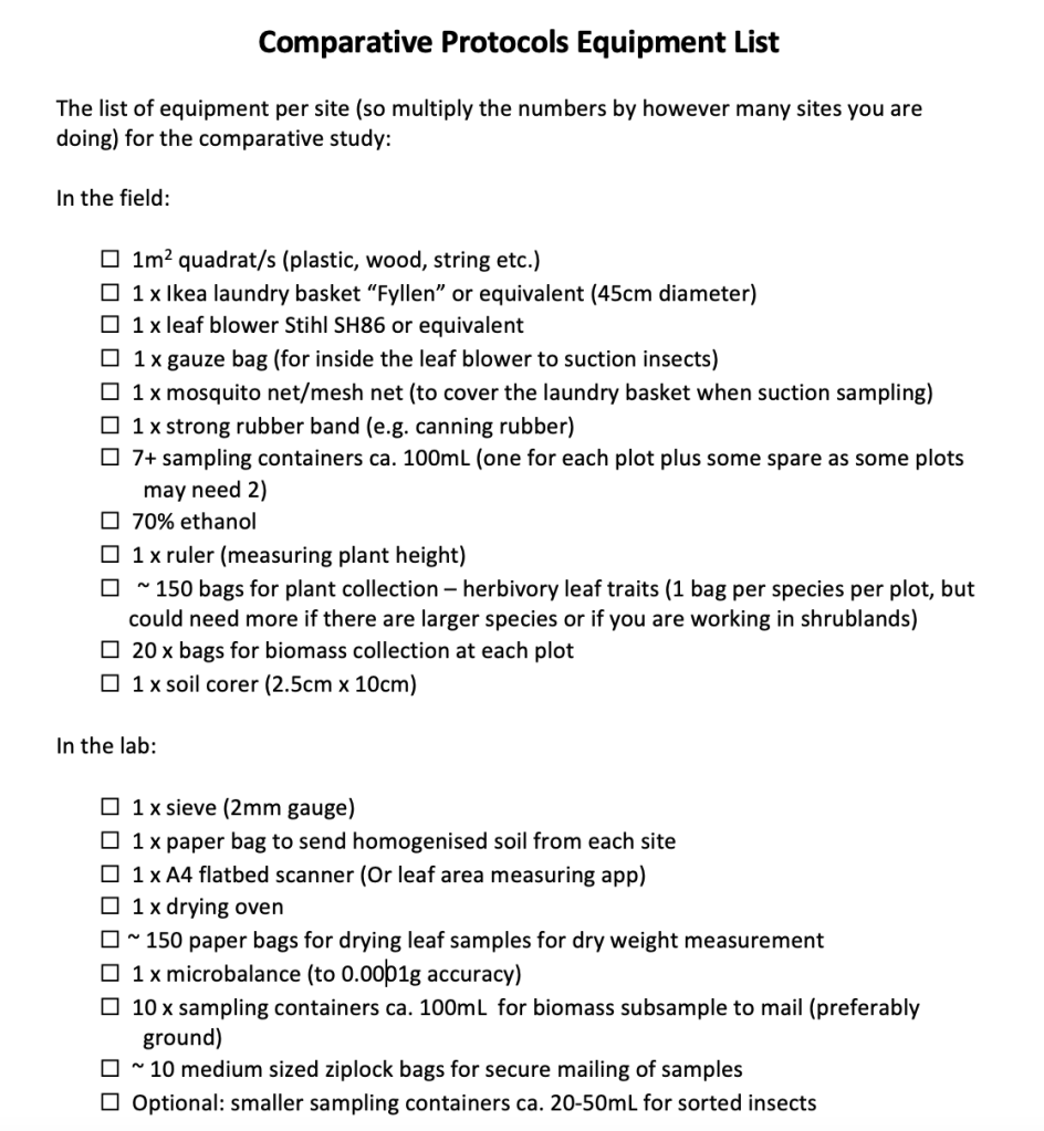
Next to seven of the ten 1m2 plots, you should cover an area of 0.16 m2 of vegetation in the middle of the plot with a cylindrical, fine-meshed gauze-cage of 45 cm diameter (Ikea laundry basket, see detailed protocol) to prevent insects from escaping. You will sample invertebrates within the cage following a standardized protocol with a leaf blower set to suction mode (Stihl SH86), equipped with a gauze-bag inserted into the suction tube. Transfer the samples to plastic containers filled with 70% ethanol. If possible, sort the invertebrates into major groups (orders, see detailed protocol), count them and classify them as herbivores or predators if possible (this will be difficult for several groups such as Heteroptera, Diptera and Coleoptera), and send them to the project coordinators for further measurements. If you will not be able to sort and classify the samples, this will be done by the project coordinators. We will provide detailed protocols on how to sample invertebrates, as well as ideas on where to find leaf blowers to borrow.
Here is a video of sampling above-ground invertebrates:
Plant species composition
Estimate the percent plant cover per plant species in each of the ten 1m x 1mplots. Cover for each plant species rooted within the plot will be estimated to the nearest 1% (up to 20% cover) and the nearest 5% for cover 20-100%. Estimate also the percent cover for woody over storey, litter, bare soil, and rocks if present. Total cover will typically exceed 100% because species cover is estimated independently for each species (see cover datasheet). To reduce bias in cover assessment, it is helpful to train yourself by placing differently sized pieces of paper on the plot: e.g. 10cm x 30cm = 3 %, 10cm x 10cm = 1 %, 3.1cm x 3.2cm = 0.1%, 31cm x 32cm = 10 % …
Herbivore damage and fungal infection
To assess herbivore damage and pathogen infection per site, you will score damage and infection in each of the 10 plots. Assess herbivore and pathogen damage species-wise.
Selection of species: Start with the species having the highest cover, followed by the species with the second highest cover, and so on, until the cover-sum of the species reaches 80% (relative cover excluding bare ground, rocks). However, do not assess damage on more than five plant species per plot. E.g. if Species A has a cover of 50%, Species B a cover of 20%, Species C a cover of 10% and Species D a cover of 8% assess damage on A, B and C. If Species A has already a cover of 90%, then only assess cover on species A. If Species A, B, C, D, and E have each a cover of 15% and species F, G, H, I… a cover of 5% then only assess damage on the five most abundant species (A,B,C,D and E) although the sum of their cover does not add up to 80%.
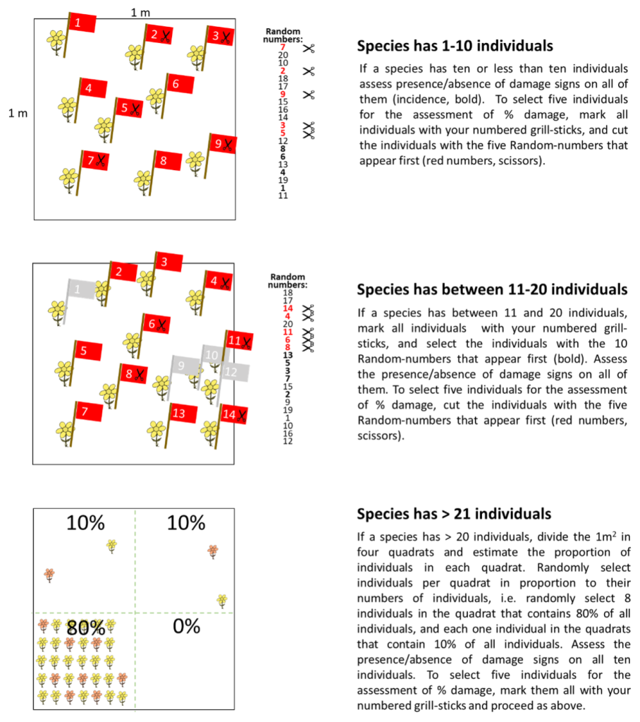
Selection of individuals per species: If your species has less than 10 individuals, select all individuals. If your species has between 10 and 20 individuals per plot, mark all individuals in the 1m2 with grill sticks numbered from 1-20. Use a random number generator (or quickly select 10 numbers in your head) to select 10 individuals (it is important that the individuals are selected randomly, and that there is no bias towards particularly damaged or undamaged ones). If your species has more than 20 individuals, divide your 1m2 plot into four quadrants, and estimate the proportion of individuals in each of the four quadrants. Randomly select individuals per quadrant in proportion to their numbers of individuals, e.g., if quadrant 1 contains 80% of all individuals, and quadrant 3 20%, then randomly select eight individuals of quadrant 1 and two of quadrant 3. Particularly if the distribution of your species is very patchy (e.g. one large patch with many individuals, and 3 isolated individuals) this methods prevents that you will select isolated individuals with a higher likelihood (see Fig. 1). Sometimes the definition of an individual is difficult as lots of plants reproduce vegetative. In this case, an individual can be defined as a ramet or branch.

Fig. 1: Selection of individuals per plant species.For each selected plant species, select 10 individuals on which you will assess the presence/absence of damage signs of the different damage categories (incidence). Of these 10 individuals you will select five individuals which you will cut at ground level (respectively a subset of them), bag, and bring to the lab for the assessment of % leaf damage and the measurements of plant traits.
For more guidance – this youtube video gives a tutorial on how to select species and individuals for damage incidence and damage % measurements.
Measurements:
On each of the selected individuals per species (max. of 10), record the presence or absence (0,1) of damage signs by chewing, mining, galling and sucking/rasping herbivores, and pathogen disease symptoms of the categories downy mildews, powdery mildews, rusts and leaf spots (see damage gallery). This will give us an estimation of damage incidence.
In addition, randomly pick five of the ten individuals (select them using the grill sticks with the first five random numbers from your random-number list), and measure the maximal height (stretch out if necessary, see section on plant traits below). Then, cut them at ground level. If your individual is very large, or builds large tussocks as is often the case for grasses, then take a subsample from the middle of the individual which contains at least five leaves. If you selected only one plant species per plot because this species had a relative cover of 80% or more, then cut all 10 individuals. On these individuals you will estimate the leaf area (%) that has been damaged. You can either do this directly in the field, or you can bag the plants in labelled plastic bags, place them in a cooler, bring them to the lab, and do the % damage assessment there. In any case, visually survey five random, mature, and non-senescing leaves (or leaflets if your leaves are very small) per individual for damage and disease symptoms. For easier inspection you can use hand lenses to better assign damage types. On each of the five leaves estimate the leaf area (%) that has been removed by chewing herbivores, mining, galling and sucking/rasping herbivores, and the leaf area that is covered by pathogenic disease symptoms of the categories downy mildews, powdery mildews, rusts and leaf spots. Some plant individuals will have fewer than 5 leaves, and for these all leaves should be surveyed (but leave out senescent leaves). Note that in some cases, damage is present on only the underside of leaves, so remember to check both sides of the leaf for damage. You can check out our detailed protocol on how to assess damage and also our photo gallery of the most common damage types.
With this method you assess damage on a minimum of 10 individuals (if one species had a cover of 80% or more) or on up to 25 individuals (if you selected 5 plant species with each 5 individuals) per plot. Five individuals per selected species and plot will be used to measure several plant leaf traits. Your bagged plants (if you do the assessment of % damage in the lab) can be used for this, see below.
UPDATE: The damage assessment is very laborious, and we realized that we slightly underestimated the time needed for this task. We therefore offer the possibility to assess the % leaf area damaged in only five instead of the ten plots. Incidence and height should be measured in all ten plots.
Shrublands:
If you work in shrublands, you may not find 10 individuals of a species in your 1m2 plot but very likely will have only one or two individuals. You may also have spreading shrubs where it can be difficult to distinguish individuals. In this case, randomly pick 50 leaves from 10 different branches per shrub species throughout the plot (5 leaves per branch). The five leaves per branch should always originate from the same leaf position, i.e. from the tip of each branch, count the first ten leaves and start sampling from there (leaf 11 to 15). Make sure that the 10 branches are from either as many shrub individuals as possible, or else take branches from different positions and orientations within the shrub patch. Assess how many of those 50 leaves are damaged. This allows us to assess the proportion of leaves that are damaged by the different damage categories per shrub individual (incidence). In addition, assess the % leaf area damaged on at least 25 randomly chosen leaves per shrub species.
If your shrub species is leafless and instead has photosynthetic stems (e.g. Retama ssp.), instead of picking leaves, randomly cut 5 cm pieces from 10 different branches throughout the plot. On these, assess how many of those pieces show damage signs of the different damage categories (incidence). In addition, on five of those branches, assess the % photosynthetic area that is damaged.
You can assess % damage either in the field or collect the leaves to assess damage in the lab. In any case you should collect a few leaves to measure several plant traits (SLA and LDMC), except on species that have photosynthetic stems where SLA and LDMC cannot be measured. These leaves for plant trait measurements should ideally not contain any damage symptoms.
UPDATE: The damage assessment is very laborious, and we realized that we slightly underestimated the time needed for this task. We therefore offer the possibility to assess the % leaf area damaged in only five instead of the ten plots. Incidence and height should be measured in all ten plots.
Plant traits
At each site, several plant traits – plant height, specific leaf area (SLA) and leaf dry matter content (LDMC) – will be measured to characterize the plant communities. These traits are closely associated to two major axis of plant functional variation, the size of plants and their parts, and the resource economics spectrum (Wright et al. 2004, Díaz et al. 2016). You will measure the traits according to protocols in Garnier et al. 2001. The traits will be measured on the same species that you have selected for the assessment of herbivore and pathogen damage. The height will be directly measured in the field, on five individuals per selected species. Use the same five individuals that you have selected for the % damage assessment. SLA and LDMC will be measured on three individuals (or subsets of the individuals) per selected species. For this, pick three or four (to have an extra one) random individuals per selected species (these can be the same individuals that you used to assess the % damage), bag them in a labelled plastic bags and place them in a cooler. If possible, your individuals have > 5 leaves without any damage symptoms, as ideally the leaf traits are measured on undamaged leaves (see detailed protocol on how to measure SLA and LDMC).
Aboveground biomass
To quantify site productivity, adjacent to each of the ten 1m x 1mplots clip the aboveground plant material to 2 cm above ground level, in two 10cm x 50cm strips (Fig. 2). Collect the total aboveground biomass, dry it for 3 days at 70 °C and weigh it. Send a subsample of the dry biomass samples to the project coordinators. If you can grind the biomass to powder, that would be ideal, but if not you can cut the biomass sample in pieces and send us a well-mixed subsample. Please send us at least 20 g of dry weight per plot (e.g. in a zip-block plastic bag or a jar, see labelling protocol). We will use the samples to measure several leaf characteristics (leaf N and P, fibre content etc.) and to identify the phyllosphere microbiome.
Shrublands:
For small shrubs, you can cut and collect the biomass as is described above. For big shrubs (> 0.5 height), divide your 1m2 plot into 4 quadrants and randomly select one quadrant. Measure the height, and canopy diameter of each shrub species in the 50 cm x 50 cm quadrant (this will be used to build allometric equations for many shrub species throughout the globe, and we are aiming to publish these results within a separate methods paper). Collect the shrub biomass that is rooted in the selected 50 cm x 50 cm quadrant, separated per shrub species, dry and weigh it (whole plant biomass). To be able to obtain a measure of shrub green vs brown biomass, please separate the leaves from the woody biomass. For some species this might work better once the leaves are dry.

Fig. 2: Sampling design per plot. For the assessment of % herbivore damage and fungal infection we will select five individuals of up to five plant species. These individuals will also be used to measure several plant traits. To assess soil characteristics, we will collect two soil cores per plot. To assess site productivity, we will sample aboveground biomass in two 10cm x 50cm strips (orange) adjacent to the plot. Next to seven of the then plots we will sample invertebrates using suction sampling.
Soil samples
Soil cores will be collected to assess a range of soil characteristics. In each of the ten plots, collect two soil cores (soil corer 2.5 x 10 cm) and homogenize the soil into a single sample per site. Please sieve the soil through a 2 mm mesh. Soils should be air-dried and send to the project coordinators (see labelling and mailing protocol sheet for more details). There, total organic C, total N and P stocks, as well as mineral N (ammonium, nitrate) and P will be measured.
1.3. Optional measurements per site
Herbivore and pathogen damage on locally rare plant species
In addition to the assessment of herbivore and pathogen damage on the most common plant species, which contribute to 80% of the relative plant cover, we will also assess the damage on the five locally most rare species per plot. This allows us to test whether locally abundant plant species usually receive more damage than locally rare ones (host concentration or dilution effect), or whether locally rare species receive more damage than locally common ones (reverse Janzen-Connell effect). To do so, start with the least abundant plant species, select 10 individuals for the assessment of damage incidence, and 5 individuals for the assessment of % leaf damage, as described above. Do the same for the second, third, fourth and fifth rarest species in the plot. You will very likely have less than 10, respectively five individuals per species. If you have sampled less than 10 individuals after the fifth species, select a sixth or seventh species until you reach 10 individuals.
Sampling of molluscs and belowground invertebrates
Assess mollusc abundance by placing a pit-fall trap baited with beer (Heineken- not because it is good but because it should be available all around the globe) next to each of five randomly chosen plots. Leave the beer-traps out for five days, but check them every two days and remove molluscs. Count the molluscs, dry and weigh them.
Pollinator assessment using pan traps
To characterise the pollinator community at a site, coloured pan trapping is considered a simple, efficient method. We will provide a standard protocol to collect flying insects at a site.
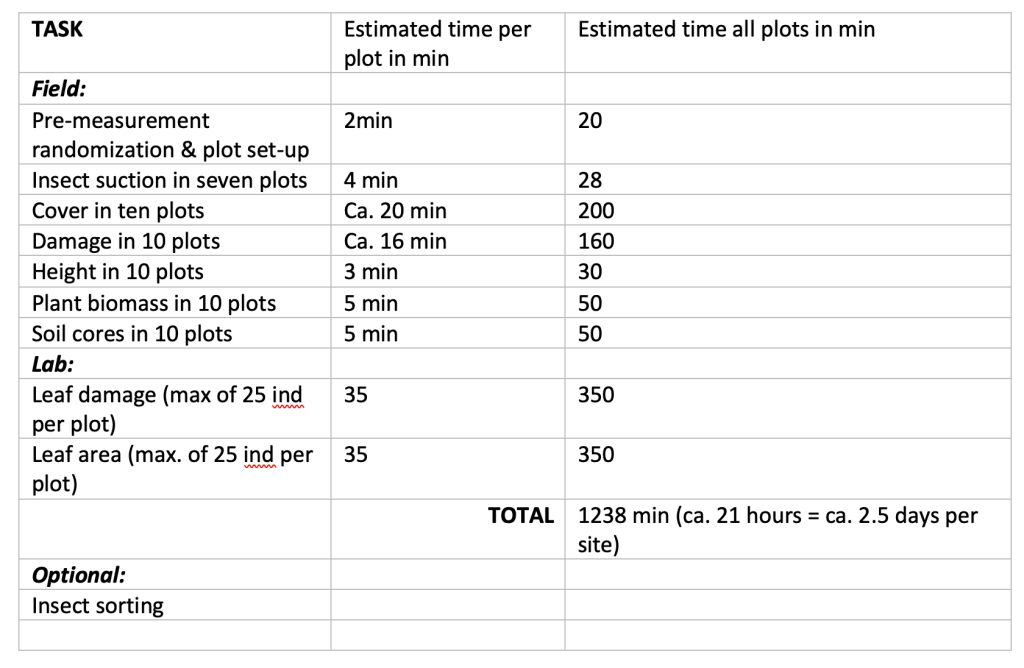
Time Estimation


